3 Inference for the multiple linear regression model
3.1 Assessing the fit
We can now formulate and fit a multiple linear regression model, and carry out a residual check to verify assumptions. However, a model can pass these checks and not be a good fit in terms of how much uncertainty in the response is accounted for by the explanatory variables, and/or the model itself may need to be simplified. Ideally, we would like a simple measure of how well our model fits the data. In a simple linear regression model we could do this by eye, i.e. a scatterplot of the data with the line of best fit overlaid, or by looking at \(R^2\). If the points lie close to the line of best fit, and \(R^2\) is large, then we have some assurance about the model.
However, this is less straightforward for multiple linear regression models, which may contain a mixture of continuous and categorical covariates, as we would have to look at multiple plots (and non-continuous covariates are less suited to this graphical approach), which might be misleading when we are primarily interested in the overall fit, i.e. the combined effect of all of the explanatory variables. Furthermore, in a simple linear regression model there is a direct equivalence between \(R^2\) and the sample correlation \(r\); this relationship does not extend to the multiple linear regression model.
One alternative approach is to use techniques from analysis of variance (anova) - which we will see again in a different context in chapter 4. We begin by considering the basic regression line concept
\[ \color{red}{\text{(observed) data} = \text{fit} + \text{residual}} \]
For a fitted multiple linear regression model this amounts to
\[\begin{align*} \color{red}{Y_i} & \color{red}{ = \hat{Y_i} + \hat{\epsilon_i}} \\ &\color{red}{= \hat{Y_i} + (Y_i - \hat{Y_i})} \end{align*}\]
for \(i = 1, \ldots, n\). To map this on to an anova-type problem, we can take the - seemingly artificial - step of subtracting the observed data mean, \(\bar{Y}\), from both sides to obtain
\[ \color{red}{Y_i - \bar{Y} = \hat{Y_i} + (Y_i - \hat{Y_i}) - \bar{Y}} \]
which can be rearranged as \[ \color{red}{(Y_i - \bar{Y}) = (\hat{Y_i} - \bar{Y}) + (Y_i - \hat{Y_i}).} \]
The first term captures the difference between an observed data point and the mean response, the second term captures the difference between a fitted data point and the mean response and the third term is the usual (unaltered) definition of the \(i^{th}\) (raw) residual.
By squaring each observation and taking the sum across each of the \(n\) observations we obtain
\[ \color{red}{\sum_{i=1}^n(Y_i - \bar{Y})^2 = \sum_{i=1}^n\left\{(\hat{Y_i} - \bar{Y}) + (Y_i - \hat{Y_i}) \right\}^2} \]
This remarkably leads to the following result
\[\begin{equation} \color{red}{\sum_{i=1}^n(Y_i - \bar{Y})^2} \color{red}{= \sum_{i=1}^n(\hat{Y}_i - \bar{Y})^2 + \sum_{i=1}^n(Y_i - \hat{Y}_i)^2} \tag{3.1} \end{equation}\]
since
\[ \color{red}{\sum_{i=1}^n (\hat{Y}_i - \bar{Y})(Y_i - \hat{Y}_i) = 0.} \]
3.2 The basic anova table
Equation (3.1) can also be stated as \[ \color{red}{\text{Total SS (TSS)} = \text{Regression SS} + \text{Residual SS}} \]
where \(\text{SS}\) refers to the sum of squares. Under an anova approach, results are typically presented and summarised in table form:
| Source | Degrees of freedom (df) | Sum of squares (SS) | Mean square (MS) | Mean square ratio (MSR) |
|---|---|---|---|---|
| Regression | \(\color{red}{p}\) | Reg SS | \(\color{red}{\text{Reg MS}\, = \frac{\text{Reg SS}}{p}}\) | \(\color{red}{F = \frac{\text{Reg MS}}{\text{RMS}}}\) |
| Residual | \(\color{red}{n - p - 1}\) | RSS | \(\color{red}{\text{RMS} = \frac{\text{RSS}}{n - p - 1}}\) | |
| Total | \(\color{red}{n - 1}\) | TSS |
So the regression model can be reduced to a single summary measure, \(F\), that can be used to test the overall significance of the model. Recall, from chapter 1, that our (unbiased) estimate of the error variance was found as
\[\begin{equation*} s^2 = \frac{\sum (y_i - \hat{y_i})^2}{n - p - 1} \end{equation*}\]
and this is exactly equivalent to the \(\text{RMS}\) in the anova table. Recall also (further back ) from MAS2902 that
\[ \frac{(N - 1)s^2}{\sigma^2} \sim \chi^2_{N - 1} \]
is the sampling distribution for the sample variance. Hence, letting \(N = n - p\) we get
\[ \frac{(n - p - 1)s^2}{\sigma^2} \sim \chi^2_{n - p - 1} \]
By recognising that we can rearrange the residual sum of squares term as \(\text{RSS} = (n - p - 1)\times\text{RMS}\) (see the anova table) we then have
\[ \frac{\text{RSS}}{\sigma^2} \sim \chi^2_{n - p - 1} \]
To find the sampling distribution of \(F\) (which we need in order to assess the significance of our result) we will make use of Cochran’s theorem.
Cochran’s Theorem
Suppose we have \(n\) observations, \(Y_i\), where \(i = 1, \ldots, n\) from the same normal distribution with mean \(\mu\) and variance \(\sigma^2\) and the total sum of squares is decomposed into \(k\) sums of squares, \(\text{SS}_{\ell}\), with associated degrees of freedom \(\nu_{\ell}\) for \(j = 1, \ldots, k\). Then, each of the sums of squares, scaled by the population variance
\[ \text{SS}_{\ell}/\sigma^2 \]
is an independent \(\chi^2\) variable with \(\nu_{\ell}\) degrees of freedom if
\[ \sum_{j = 1}^k \nu_{\ell} = n - 1. \]
In our case, we have broken the total sum of squares for our multiple linear regression model into two components, Reg SS and RSS. The observations will have the same mean when all the \(\beta\) parameters are simultaneously zero, which we can use as a null hypothesis (see later). Each observation has the same variance, \(\sigma_\epsilon^2\) in our case (this is one of our key assumptions), and the respective degrees of freedom are \(p\) (for Reg SS) and \(n - p - 1\) (for RSS) and these sum to \(n - 1\).
Thus, applying Cochran’s theorem, we must have that
\[ \color{red}{\text{Reg SS}/\sigma_{\epsilon}^2} \]
is an independent \(\chi^2\) variable, with \(p\) degrees of freedom, since
\[ \color{red}{\text{RSS}/\sigma_{\epsilon}^2} \]
is also an independent \(\chi^2\) variable, with \(n - p - 1\) degrees of freedom (we already demonstrated this). When we form our \(F\) statistic we divide Reg MS by RMS, i.e. we form the mean square ratio (MSR) which we denote by \(F\):
\[ \color{red}{F = \frac{\text{Reg MS}}{\text{RMS}}} \]
Both of these quantities are a sum of squares divided by its associated degrees of freedom, hence
\[ \color{red}{F = \frac{\left(\frac{\text{Reg SS}}{p}\right)}{\left(\frac{\text{RSS}}{n - p - 1}\right)}} \]
We can divide the top and bottom by \(\sigma_{\epsilon}^2\) to ensure the numerator and denominator are both \(\chi^2\) quantities
\[ \color{red}{F = \frac{\left(\frac{\text{Reg SS}/\sigma_{\epsilon}^2}{p}\right)}{\left(\frac{\text{RSS}/\sigma_{\epsilon}^2}{n - p - 1}\right)} \sim F_{p, n - p - 1}} \]
Why do we do this? The F-distribution arises as a ratio of scaled, independent \(\chi^2\) variables, and this is exactly what we now have above. Hence \(F\) in our anova table provides us with a means of testing
\[ \color{red}{H_0: \beta_1 = \beta_2 = \ldots = \beta_p = 0} \]
versus
\[ \color{red}{H_1: \text{at least one}\; \beta_j \neq 0, j = 1, \ldots, p.} \]
This is an example of an omnibus test and we use the test statistic above, \(F = \text{Reg MS}/\text{RMS}\). When the values of \(F\) are large (why?) we reject the null hypothesis, \(H_0\), in favour of the alternative hypothesis, \(H_1\) and we judge this using \(p\)-values as before. Note that both the total sum of squares (TSS) and the total degrees of freedom are unaffected by model choice since these are fixed quantities from the data.
The coefficient of determination
A widely-used summary measure of the performance of the regression is the coefficient of determination (or correlation), \(R^2\), where
\[ \color{red}{R^2 = \frac{\text{Reg SS}}{\text{TSS}} = 1 - \frac{\text{RSS}}{\text{TSS}}.} \]
This can be interpreted as the proportion of the corrected sum of squares that is explained by the candidate model, i.e. the proportion of the variability in the response that is explained by the explanatory variables. The range of \(R^2\) is zero to one but it is often expressed as a percentage to aid interpretation.
Example: Cheddar cheese study
As cheddar cheese matures, a variety of chemical processes take place. The taste of matured cheese is related to the concentration of several chemicals in the final product. In a study of cheddar cheese from several regions in the UK, 30 samples of cheese were analyzed for their chemical composition and were subjected to taste tests. Data from the study are available in the file cheese.RData with the following variables:
- Taste: a combined score obtained from several tasters with higher scores indicating tastier cheese (the variable);
- H2S: the natural log of the concentration of hydrogen sulfide;
- Lactic: the concentration of lactic acid.
| Taste | H2S | Lactic |
|---|---|---|
| 57.2 | 7.908 | 1.90 |
| 56.7 | 10.199 | 2.01 |
| 54.9 | 6.752 | 1.52 |
| 47.9 | 7.496 | 1.81 |
| 40.9 | 9.588 | 1.74 |
For these data we can fit a multiple linear regression model
\[ \color{red}{\text{Taste}_i = \beta_0 + \beta_1\text{H2S}_i + \beta_2\text{Lactic}_i + \epsilon_i} \]
for \(i = 1, \ldots, 30\), and with the usual assumptions about \(\epsilon_i\) of normality, independence and a common variance. Construct an anova table and test the overall significance of the model.
Solution
We have \(n = 30\) here, and can calculate the total sum of squares from the raw data. We then use the `lm’ command to fit a model in the usual way before extracting the residual sum of squares, the regression sum of squares are then obtained by subtraction; note that both of these quantities depend on the fitted model. Now \[\begin{align*} \color{red}{\textrm{TSS}} &\color{red}{= \sum_{i=1}^{30} (y_i - \bar{y})^2} \\ &\color{red}{= \sum_{i=1}^{30} y_i^2 - 30\bar{y}^2} \\ &\color{red}{= (57.2^2 + 56.7^2 + \ldots ... + 0.7^2) - 30 \times 24.53^2} \\ &\color{red}{= 7662.887} \end{align*}\]
We can then fit a regression model in the usual way, before extracting the residual sum of squares as follows:
## [1] 2668.965We can now produce the anova table for this model:
| Source | df | SS | MS | MSR |
|---|---|---|---|---|
| \(\color{red}{\text{Regression}}\) | \(\color{red}{2}\) | \(\color{red}{4993.921}\) | \(\color{red}{2496.961}\) | \(\color{red}{25.260}\) |
| \(\color{red}{\text{Residual}}\) | \(\color{red}{27}\) | \(\color{red}{2668.965}\) | \(\color{red}{98.851}\) | |
| \(\color{red}{\text{Total}}\) | \(\color{red}{29}\) | \(\color{red}{7662.887}\) |
Clearly, we have a large F-statistic. Comparing with \(F_{2, 27}\) (why?) in tables we see that \(p < 0.01\) and we clearly reject the null hypothesis that \(\beta_1 = \beta_2 = 0\). We can also calculate \[ \color{red}{R^2 = \frac{4993.921}{7662.887} = 0.6517} \]
Thus, around two-thirds of the variation has been explained, but this does not necessarily mean this is the right model. The (omnibus) \(F\)-test considers all the coefficients together and a significant result indicates that at least one of them is non-zero, but which one, or is it both? In order to answer this question we also need a procedure to consider the coefficients separately. We first, however, take a detour and demonstrate how to fully construct an anova table using R, although it is a slightly clunky procedure.
Anova in R
We can fit the model in R in the usual way and then use the anova() command to get the sum of squares breakdown via the following commands:
## Analysis of Variance Table
##
## Response: Taste
##           Df Sum Sq Mean Sq F value    Pr(>F)
## H2S        1 4376.7  4376.7 44.2764 3.851e-07 ***
## Lactic     1  617.2   617.2  6.2435   0.01885 *
## Residuals 27 2669.0    98.9
## ---
## Signif. codes:  0 '***' 0.001 '**' 0.01 '*' 0.05 '.' 0.1 ' ' 1
We get the (rounded) residual sum of squares directly (\(RSS = 2669\)), but a breakdown of the regression sum of squares rather than the total value, although we can easily get the total by addition, i.e. \(\text{Reg SS} = 4376.7 + 617.2 = 4993.9\).
N.B. What we actually get is the Type I sums of squares, where the order variables are entered matters, as opposed to Type II sums of squares which condition on the other variables and are thus independent of order.
The F-statistic can be found in R using the last line of the output from
##
## Call:
## lm(formula = Taste ~ H2S + Lactic, data = cheese)
##
## Residuals:
##     Min      1Q  Median      3Q     Max
## -17.343  -6.530  -1.164   4.844  25.618
##
## Coefficients:
##             Estimate Std. Error t value Pr(>|t|)
## (Intercept)  -27.592      8.982  -3.072  0.00481 **
## H2S            3.946      1.136   3.475  0.00174 **
## Lactic        19.887      7.959   2.499  0.01885 *
## ---
## Signif. codes:  0 '***' 0.001 '**' 0.01 '*' 0.05 '.' 0.1 ' ' 1
##
## Residual standard error: 9.942 on 27 degrees of freedom
## Multiple R-squared:  0.6517, Adjusted R-squared:  0.6259
## F-statistic: 25.26 on 2 and 27 DF,  p-value: 6.551e-07
Hence \(F = 25.26\) in this case - as in our anova table, with an exact p-value of \(6.551 \times 10^{-7}\). We can also obtain \(R^2\) from the penultimate line of the output, or directly using
## [1] 0.6517024which again matches what we found earlier. Hence, we can use R to circumvent the need for a formal anova table since both \(F\) and \(R^2\) can be easily extracted.
3.3 The extra sum of squares method
Suppose we fit a multiple linear regression model with two continuous covariates: \[ Y_i = \beta_0 + \beta_1 x_{i1} + \beta_2 x_{i2} + \epsilon_i. \] How should we decide if either of the explanatory variables adds anything to the model? The easiest way is to fit the model with and without the variable and observe the change in the model sum of squares. We can test this change using the `extra sum of squares’ principle. Helpfully, we can use an anova table - similar to those seen earlier - by including an additional row to the basic table.
3.3.1 The extended anova table
The regression sum of squares is broken down in to its contribution from each covariate. A key feature of this method is that the order that the covariates are entered into the model matters, as we shall see in the following examples. The general table structure is given below:
Note that \(\text{Reg SS}_{x_1 + x_2}\) is the regression sum of squares from the full model.
| Source | df | SS | MS | MSR |
|---|---|---|---|---|
| Regression on \(x_1\) | 1 | \(\text{Reg SS}_{x_1}\) | \(\text{Reg MS}_{x_1}=\text{Reg SS}_{x_1}\) | \(F_1 = \frac{\text{Reg MS}_{x_1}}{\text{RMS}}\) |
| Regression on \(x_2\) having fitted \(x_1\) | 1 | \(\text{Reg SS}_{x_2 \mid x_1} =\) \(\text{Reg SS}_{x_1 + x_2} - \text{Reg SS}_{x_1}\) |
\(\text{Reg MS}_{x_2 \mid x_1}=\text{Reg MS}_{x_2 \mid x_1}\) | \(F_2= \frac{\text{Reg MS}_{x_2 \mid x_1}}{\text{RMS}}\) |
| Residual | \(n - 3\) | RSS | \(\text{RMS} = \frac{\text{RSS}}{n - 3}\) | |
| Total | \(n - 1\) | TSS |
Note that \(\text{Reg SS}_{x_1 + x_2}\) is the regression sum of squares from the full model.
Example: Extra sum of squares for cheese data
Returning to the cheese data, we can fit the model with either hydrogen sulfide or lactic acid first, i.e. there are two possible orderings. As order matters in the extra sum of squares method we will consider both possibilities in turn to investigate any possible differences.
To produce anova tables for the extra sum of squares approach we can use the generic R command anova() as a basis, albeit with some additional work involved to construct the anova table. Fitting hydrogen sulfide first, we get:
## Analysis of Variance Table
##
## Response: Taste
##           Df Sum Sq Mean Sq F value    Pr(>F)
## H2S        1 4376.7  4376.7 44.2764 3.851e-07 ***
## Lactic     1  617.2   617.2  6.2435   0.01885 *
## Residuals 27 2669.0    98.9
## ---
## Signif. codes:  0 '***' 0.001 '**' 0.01 '*' 0.05 '.' 0.1 ' ' 1
We can thus populate the anova table:
| Source | df | SS | MS | MSR |
|---|---|---|---|---|
| Regression on H2S | 1 | 4376.746 | 4376.746 | 44.276 |
| Regression on lactic acid having fitted H2S | 1 | 617.176 | 617.176 | 6.244 |
| Residual | 27 | 2668.965 | 98.851 | |
| Total | 29 | 7662.887 |
Since \(F_{1, 27}(5\%) = 4.21\) we can see that H2S is needed in the model since \(F_1 = 44.276\) hugely exceeds this critical value (the exact p-value from R is \(3.851 \times 10^{-7}\)). We also see that \(F_2 = 6.244\) exceeds the critical value, so lactic acid is needed in the model, after H2S has already been included (from R, \(p = 0.01885\)). The model where we switch the order of the variables can be fitted in R using
## Analysis of Variance Table
##
## Response: Taste
##           Df Sum Sq Mean Sq F value   Pr(>F)
## Lactic     1 3800.4  3800.4  38.446 1.25e-06 ***
## H2S        1 1193.5  1193.5  12.074 0.001743 **
## Residuals 27 2669.0    98.9
## ---
## Signif. codes:  0 '***' 0.001 '**' 0.01 '*' 0.05 '.' 0.1 ' ' 1
This leads to the anova table below:
| Source | df | SS | MS | MSR |
|---|---|---|---|---|
| Regression on lactic acid | 1 | 3800.398 | 3800.398 | 38.446 |
| Regression on H2S having fitted lactic acid | 1 | 1193.523 | 1193.523 | 12.074 |
| Residual | 27 | 2668.965 | 98.851 | |
| Total | 29 | 7662.887 |
We can see that both \(F_1\) and \(F_2\) are comfortably bigger than our critical value of 4.21 (this is still the same value) so conclude that lactic acid is needed in the model, and that hydrogen sulfide is needed in the model after lactic acid has been included. The conclusion is unambiguous here: both variables are needed in the model, irrespective of ordering. Note that the residual and total SS are unaffected by the ordering (this is also true for the critical value).
We now consider another example where the conclusion is not so clear cut. Henceforth, we will use R directly without formally constructing anova tables.
Example: Warfarin study
Children with heart problems take warfarin to avoid getting strokes. In a study of 120 children, the warfarin dose (mg), age (months) and height (cm) were measured. A scatterplot of the dose against age produced the following plot
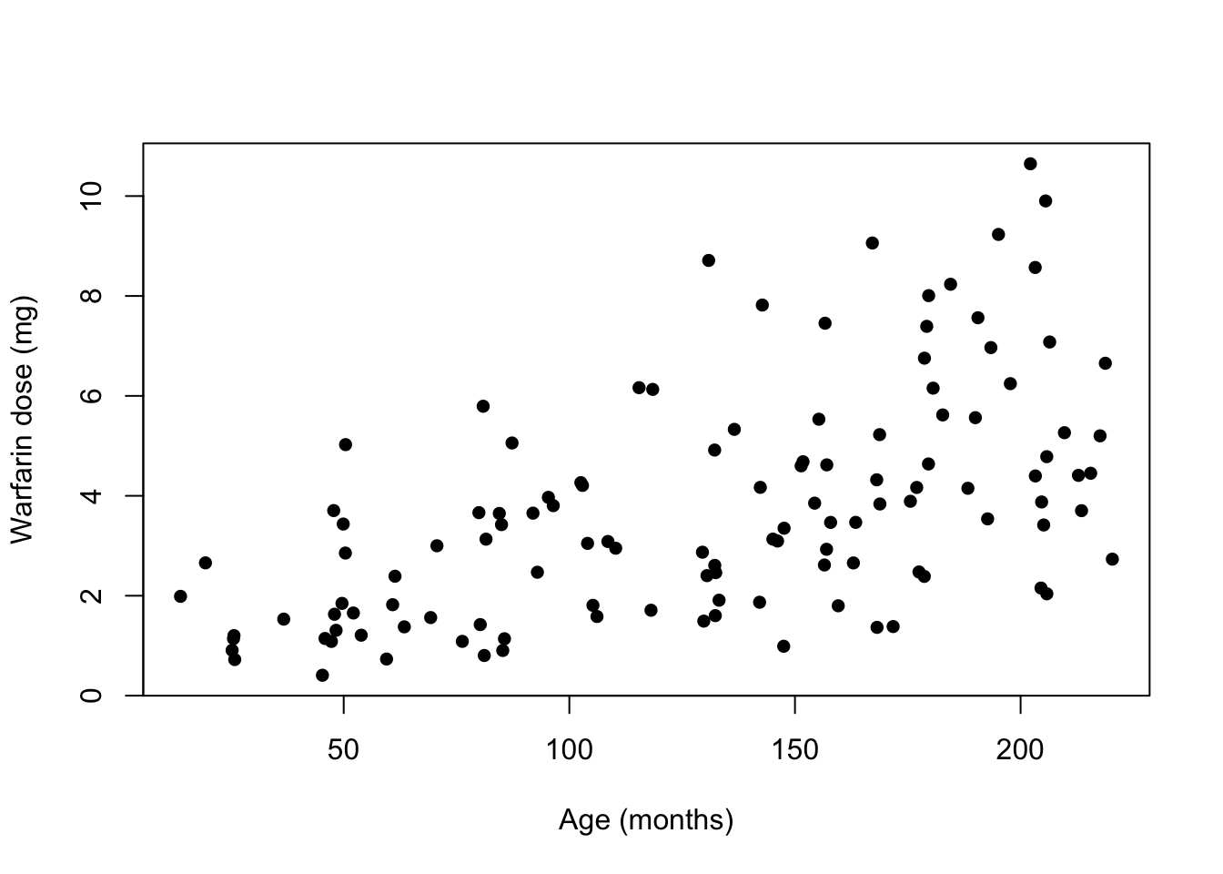
Figure 3.1: Scatterplot of dose against age for the warfarin study.
The average dose increase with age but so does the variability (spread of observations). The latter breaks one of our assumptions! We need to transform the dose to stabilise the variance (we will return to transformations formally later in the semester). Here we take the square root transformation (other transformations may also work as well, or better) which has the effect of reducing the larger values (more than the smaller values due to the nature of the square root operator). The original variable is in the R dataframe warfarinStudy, so we can perform the transformation using
# Add the new variable to the data frame
warfarinStudy$root_dose = sqrt(warfarinStudy$warfarin_dose)
Plotting the square root of dose against age we see that it increases on average with increasing age and that the variability is now approximately constant.
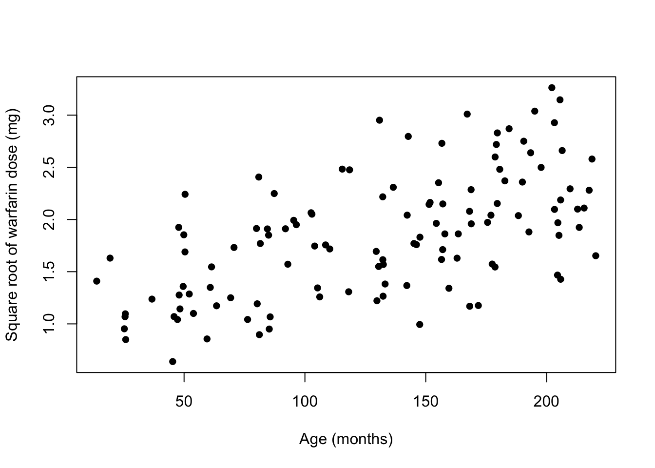
Figure 3.2: Scatterplot of the square root of dose against age for the warfarin study.
A similar picture is obtained if we plot the square root of dose against height (the other possible covariate here). We shall now regress the square root of dose against height and age, looking at both possible orderings. The R command anova() breaks down the regression sum of squares into its individual contribution from each covariate:
## Analysis of Variance Table
##
## Response: root_dose
##            Df Sum Sq Mean Sq F value    Pr(>F)
## height      1 13.046 13.0462 58.4899 6.289e-12 ***
## age         1  1.152  1.1520  5.1647   0.02488 *
## Residuals 117 26.097  0.2231
## ---
## Signif. codes:  0 '***' 0.001 '**' 0.01 '*' 0.05 '.' 0.1 ' ' 1
Height on its own produces a miniscule p-value (\(6.289 \times 10^{-12}\)) and thus we clearly need to include height. Fitting age height also gives a small p-value (\(0.025 < 0.05\)) which implies that we also need age, once height has been fitted.
In a similar way we can again use the command anova() for a model that includes age first, followed by height.
## Analysis of Variance Table
##
## Response: root_dose
##            Df  Sum Sq Mean Sq F value    Pr(>F)
## age         1 14.1975 14.1975  63.652 1.124e-12 ***
## height      1  0.0007  0.0007   0.003    0.9564
## Residuals 117 26.0969  0.2231
## ---
## Signif. codes:  0 '***' 0.001 '**' 0.01 '*' 0.05 '.' 0.1 ' ' 1
Age on its own produces a very small p-value (\(1.124 \times 10^{-12}\)) and thus we clearly need to include age. Fitting height after age gives a non-significant p-value (\(0.9564 > 0.05\)), however, which implies that we do not need height once age has been fitted.
Thus we have conflicting conclusions (for height) - model one suggests we do need height, model two indicates that we do not; both models unanimously agree that age is needed. We want as simple model as possible and so we should just include age and then do model checking as described in chapter 2.
Why has this happened? The problem has arisen because age and height are highly correlated. We shall come back to this problem later. The correlation is in fact 0.95 (see plot).
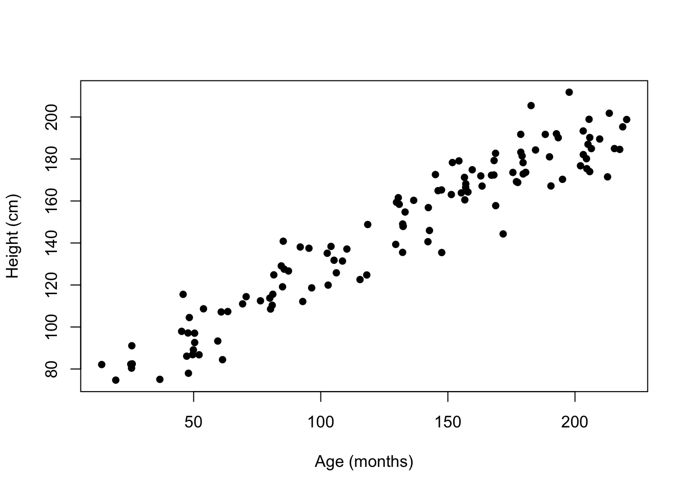
Figure 3.3: Scatterplot of height against age for the warfarin study.
3.4 The general extra sum of squares method
The extra sum of squares method is most useful if we wish to test whether a subset of the explanatory variables have no effect on the response variable. This can help simplify the model by removing several covariates at once - it is also useful for dealing with factors that have several levels, such as eye colour or favoured mode of transport.
In order to use the extra sum of squares method in this scenario we order the \(x\) variables so that the subset we are going to test takes the last \(q\) places of the parameter vector \(\underline{\beta}\). Notationally, we partition the parameter vector as
\[\begin{align*} \color{red}{\underline{\beta} = \begin{pmatrix} \underline{\beta}_1 \\ \underline{\beta}_2 \\ \end{pmatrix}} \end{align*}\]
where \(\underline{\beta}_2\) is the \(q-\)vector of parameters that we wish to consider for removal from the model, and \(\underline{\beta}_1\) is the \((p-q)\)-vector of parameters which we wish to keep in the model.
To carry out the procedure, we firstcalculate (usually using R) the regression sum of squares for fitting all \(p\) candidate parameters, i.e. fit the full (additive) model. We then calculate (again using R, typically) the regression sum of squares for fitting the \(p - q\) parameters which we want to include, i.e. fit the subset model. We can then form an extended general anova table:
| Source | df | SS | MS | MSR |
|---|---|---|---|---|
| Regression on \(x_1, \ldots x_{p-q}\) | \(p - q\) | \(\text{Reg SS}_{\underline{\beta}_1}\) | \(\text{Reg MS}_{\underline{\beta}_1}=\frac{\text{Reg SS}_{\underline{\beta}_1}}{p-q}\) | \(F_1 = \frac{\text{Reg MS}_{\underline{\beta}_1}}{\text{RMS}}\) |
| Regression on \(x_{p-q+1}, \ldots x_p\) having fitted \(x_1, \ldots x_{p-q}\) | \(q\) | \(\text{Reg SS}_{\underline{\beta}_2 \mid \underline{\beta}_1} =\) \(\text{Reg SS}_{\underline{\beta}} - \text{Reg SS}_{\underline{\beta}_1}\) |
\(\text{Reg MS}_{\underline{\beta}_2 \mid \underline{\beta}_1}=\frac{\text{Reg MS}_{\underline{\beta}_2 \mid \underline{\beta}_1}}{q}\) | \(F_2= \frac{\text{Reg MS}_{\underline{\beta}_2 \mid \underline{\beta}_1}}{\text{RMS}}\) |
| Residual | \(n - p - 1\) | RSS | \(\text{RMS} = \frac{\text{RSS}}{n - p - 1}\) | |
| Total | \(n - 1\) | TSS |
We can now test \(H_0: \beta_{p - q + 1} = \beta_{p - q + 2} = \ldots = \beta_p = 0\) given that \(\beta_1, \ldots, \beta_{p - q}\) have been included in the model using \(F_2\). This is tested against a general alternative \(H_1: \text{at least one}\;\; \beta_j \neq 0\) for \(j = p - q + 1, \ldots, p\). This is another example of an test as we are testing for several things simultaneously. Large values of \(F_2\) lead to rejection of the null hypothesis, \(H_0\). This process allows us to remove a block of parameters from a model, rather than one-by-one, and is particularly useful when adding parameters to a model where previous research or expert knowledge suggests some covariates must be included in the model. In essence, we are then testing whether the extra covariates can add anything to the established model.
Example: Extended extra sum of squares for cheese data
Returning to the cheese data, three additional variables are also available in the dataset cheese2.RData, namely
- Acetic: the natural log of the concentration of acetic acid (in micromoles per liter, \(\mu\)mol/L);
- Phosphoric: the amount of phosphoric acid (in mg);
- Citric: the amount of citric acid (in ml).
We can use the extra sum of squares method to investigate whether these additional variables should be added to the original model containing H2S and lactic acid. We do so by fitting the full model and the reduced model with the first \(p\) parameters included (we do not need to fit a model with just the remaining parameters). As usual, we can make repeated use of lm() to do this:
load("cheese2.RData")
fit1 = lm(Taste ~ H2S + Lactic, data = cheese2)
fit2 = lm(Taste ~ ., data = cheese2)
# Using . fits every variable in the dataset as a predictor
We can then use the anova command with two arguments (which must be nested models) to carry out the extra sum of squares method and test whether any of acetic, phosphoric or citric acid are needed in the model. The R command and output is shown below:
## Analysis of Variance Table
##
## Model 1: Taste ~ H2S + Lactic
## Model 2: Taste ~ H2S + Lactic + Acetic + Phosphoric + Citric
##   Res.Df    RSS Df Sum of Sq      F Pr(>F)
## 1     27 2669.0
## 2     24 2602.5  3    66.484 0.2044 0.8923
The syntax is such that we should always have the reduced model first, i.e.
We see that \(p = 0.8923 > 0.05\) so we can retain the null hypothesis and our original model containing both H2S and lactic acid is our chosen model; acetic, phosphoric and citric acid are not needed in the model, in the presence of H2S and lactic acid.
Summary: extra sum of squares method
Removing several parameters at once can lead to the removal of potentially important predictors. This can happen if one variable is borderline significant and the others are not. Hence, we should proceed cautiously. The method must be used for factors with more than two levels since we need a way of assessing the overall significance of the variable which cannot be done using parameter-specific \(p\)-values - see later chapters. For a solitary continuous (or ordinal) covariate (or a factor with 2 levels) - i.e. anything with a solitary degree of freedom - we can still apply the method, but it is slightly inefficient, as we shall see in section ??.
Example: Anova for crime data based on summary information
A dataset consisting of crime rates from 47 US states along with 13 continuous explanatory variables was analysed in R using an additive multiple linear regression model. An incomplete analysis of variance using all thirteen predictors produced the following table:
| Source | df | SS | MS | MSR |
|---|---|---|---|---|
| Regression on all predictors | 52931 | |||
| Residual | 15879 | |||
| Total | 46 | 68810 |
- Complete the anova table and test for significance for all 13 predictors simultaneously.
-
A criminologist postulates that there are five key drivers of state crime and conducts a multiple linear regression model using these five covariates. The parameter estimates (and their standard errors) are given below.
Which variable appears to be the most important? Which seems to be the least important?Estimate Standard error 1.02 0.35 2.03 0.47 1.23 0.14 0.91 0.43 0.63 0.14 - The data analyst further reports that the residual sum of squares is \(18604\) for the reduced model. Use this information to test whether the criminologist’s model is sufficient for these data. [You are not required to produce the formal anova table.]
- Compare the values of \(R^2\) for the full model and that put forward by the criminologist.
Solution
-
Since we have 13 continuous predictors we must have 13 degrees of freedom for the regression. Then, by subtraction, we can get the error degrees of freedom as \(46 - 13 = 33\).
Once we have the sums of squares and their associated degrees of freedom it is easy to calculate the mean square terms working within rows. For the regression we have \(52931/13 = 4071.615\) and for the error \(15879/33 = 481.82\). Finally, we calculate the test statistics as the ratio of the regression mean square to the error mean square, i.e. \(4071.615/481.182 = 8.462\). This completes the anova table.
Source df SS MS MSR Regression on all predictors 13 52931 4071.615 8.462 Residual 33 15879 481.82 Total 46 68810 We can look up the \(5\%, 1\%\) and \(0.1\%\) critical values in
Rusingqf(c(0.95, 0.99, 0.999), 13, 33)to get 2.030, 2.723 and 3.773 respectively. Since \(8.462 > 3.773\) we conclude that at least one of the predictors is important and there is very strong evidence of some relationship between crime rate and the explanatory variables.
-
To answer this question we must take the ratios to get the respective \(t\)-statistics. This gives
Hence, we can now say that \(x_3\) is the most important predictor, followed by \(x_5\) (which had the lowest estimate). The least important predictor is \(x_4\), although it still has a reasonably large \(t\)-valueEstimate Standard error t 1.02 0.35 2.914 2.03 0.47 4.319 1.23 0.14 8.786 0.91 0.43 2.116 0.63 0.14 4.5 -
Using the relation that the total SS is the sum of the regression and residual SS terms we can get the regression SS for the five-predictor model as \(68810 - 18604 = 50206\). To test the reduced model we need its (conditional) regression sum of squares, found by subtraction as \(52931 - 50206 = 2725\) (note that \(52931\) is the regression sum of squares from the full model in (a)).
This has 8 degrees of freedom associated so the regression MS for the additional 8 variables is \(2725/8 = 340.625\) which we compare to the full model error MS to get \(F = 340.625/481.182 = 0.71\). FromR, \(F_{8, 33}(5\%) = 2.235\) so we retain the null hypothesis - the extra 8 predictors are not needed if the five variables nominated by the criminologist are already in the model.
A more direct solution is to note that the difference in the residual sums of squares will also give us the reduced model SS, namely \(18604 - 15879 = 2725\). We then proceed as above. - To calculate \(R^2\) we divide the regression total sum of squares by the total sum of squares to identify how much of the total is explained by the regressors. In this case \(R^2 = 52931/68810 = 0.769\), so all of the predictors combined explain around \(77\%\) of the variability in crime rates. For the pathologist’s model \(R^2 = 50206/68810 = 0.730\), i.e. around \(73\%\) of the variability. This is not much different for the loss of eight predictors and suggests there is some validity to the claim.
3.5 Confidence and prediction intervals for the fitted values
Recall that the fitted values in a mutliple linear regression model are given by
\[\begin{align*} \underline{\hat{Y}} &= \mathrm{X}\underline{\hat{\beta}} \\ &= \mathrm{X}(\mathrm{X}^T\mathrm{X})^{-1}\mathrm{X}^T\underline{Y} \\ &= \mathrm{H}\underline{Y} \end{align*}\]
Making use of these alternative forms we found the expectation and the variance of the fitted values back in subsection 1.4.4 of the notes, namely
\[ \mathrm{E}[\underline{\hat{Y}}] = \mathrm{X}\underline{\beta} \]
and
\[\begin{equation*} \mathrm{Var}[\underline{\hat{Y}}] = \mathrm{H}\sigma_{\epsilon}^2. \end{equation*}\]
Hence, at the individual observation level, we have \(\mathrm{E}\left[\hat{Y}_i\right] =\underline{x}_i^T \underline{\beta}\). Also, for the variance we have \(\mathrm{Var}\left[\hat{Y}_i\right] = h_{ii}\sigma_{\epsilon}^2\) for \(i = 1, \ldots, n\), where the \(h_{ii}\) are the diagonal elements (the leverages, recall) of the hat matrix \(\mathrm{H}\). By noting that the fitted values are a linear combination of random variables, \(\underline{\hat{\beta}}\), we can see that they are also normally distributed. This means we can find a \(100(1 - \alpha)\%\) confidence interval for the fitted value in the usual way as
\[ \hat{Y}_i \pm t_{\nu, 1 - \alpha/2} \times s \sqrt{h_{ii}} \]
where \(\nu = n - p - 1\) is the residual degrees of freedom and \(s\) is the square root of RMS (see earlier).
It is instructive at this point to consider how the individual \(h_{ii}\) terms are calculated. Clearly, from a fitted model object we can just extract them using the R command hatvalues(), but what about for a new observation? Consider the variance of the fitted value, \(\hat{Y}_p\), for this new observation, with covariate vector \(\underline{x}_p\):
\[\begin{align*} \color{red}{\mathrm{Var}\left[\hat{Y}_p\right]} &\color{red}{= \mathrm{Var}\left[\underline{x}_p^T \underline{\hat{\beta}}\right]} \\ &\color{red}{= \underline{x}_p^T \mathrm{Var}\left[\underline{\hat{\beta}}\right] \underline{x}_p} \\ &\color{red}{= \underline{x}_p^T (\mathrm{X}^T\mathrm{X})^{-1} \underline{x}_p \sigma_{\epsilon}^2} \end{align*}\]
Hence, for any (observed or typically new) covariate pattern \(\underline{x}_p\) we can calculate the confidence interval for the fitted response as
\[ \color{red}{\hat{Y}_p \pm t_{\nu, 1 - \alpha/2} \times s \sqrt{h_{pp}}} \]
where \(h_{pp} = \underline{x}_p^T (\mathrm{X}^T\mathrm{X})^{-1} \underline{x}_p\). Note that this interval is for the average or mean response, i.e. for observations that lie perfectly on the line of best fit and have no error attached to them. To account for error, we can also calculate a prediction interval for an individual observation, based on a vector of covariates, again either observed or, more likely, new. We now have \[\begin{align*} \color{red}{\hat{Y}_p^*} &\color{red}{= \underline{x}_i^T \underline{\hat{\beta}} + \epsilon_p} \\ &\color{red}{= \hat{Y}_p + \epsilon_p} \end{align*}\]
where \(\epsilon_p\) captures the unknown error associated with the prediction, and is assumed to be normally distributed, and independent of \(\hat{Y}_p\). Hence,
\[\begin{align*} \color{red}{\mathrm{Var}\left[\hat{Y}_p^* \right]} &\color{red}{= \mathrm{Var}\left[\underline{x}_p^T \underline{\hat{\beta}}\right] + \mathrm{Var}[\epsilon_p]} \\ &\color{red}{= \underline{x}_p^T (\mathrm{X}^T\mathrm{X})^{-1} \underline{x}_p\sigma_{\epsilon}^2 + \sigma_{\epsilon}^2} \\ &\color{red}{= \left(\underline{x}_p^T (\mathrm{X}^T\mathrm{X})^{-1} \underline{x}_p + 1\right) \sigma_{\epsilon}^2}, \end{align*}\]
and a prediction interval for a new observation is found as \[ \color{red}{\hat{Y}_p^* \pm t_{\nu, 1 - \alpha/2} \times s \sqrt{h_{pp} + 1}.} \]
Note the distinction between the two intervals - the prediction interval is always wider. The prediction interval is the interval for an actual observation, whereas the confidence interval is for the average observation, both based on the same set of covariate values. In each case, the width of the interval increases with the leverage - high leverage points are predicted less accurately.
Example: Confidence and prediction intervals for the cheese data
Confidence and prediction intervals for the fitted values can be easily calculated using R. We need a fitted model (obviously!) and a dataframe containing the covariate values for which we want to construct our confidence and prediction intervals - this is best seen by example. Thus, for the original cheese example with just two covariates:
fit1 = lm(Taste ~ H2S + Lactic, data = cheese)
newdat = data.frame(H2S = 6, Lactic = 1.5)
predict(fit1, newdat, interval = "confidence")
## fit lwr upr
## 1 25.9166 22.09274 29.74045## fit lwr upr
## 1 25.9166 5.161269 46.67192The prediction interval is much wider, by a factor of about 5 for these values of the explanatory variables.
3.6 Polynomial models
Sometimes the response might have a curvilinear relationship with one or more of the explanatory variables and we may think about fitting a polynomial model - remember that this still falls under our multiple linear regression framework as long as the postulated model is linear in the parameters, \(\underline{\beta}\). For instance, if there is just one explanatory variable we might consider fitting
\[ \color{red}{Y_i = \beta_0 + \beta_1 x_i + \beta_2 x_i^2 + \beta_3 x_i^3 + \epsilon_i} \]
for \(i = 1, \ldots, n\). Defining
\[ \color{red}{x_{i1}^* = x_i; x_{i2}^* = x_i^2; x_{i3}^* = x_i^3}, \]
the model then becomes
\[ \color{red}{Y_i = \beta_0 + \beta_1 x_{i1}^* + \beta_2 x_{i2}^* + \beta_3 x_{i3}^* + \epsilon_i} \]
which is of exactly the form of a multiple linear regression model. Other covariates can also be included in the usual way, i.e.
\[ \color{red}{Y_i = \beta_0 + \beta_1 x_{i1} + \beta_2 x_{i2} + \beta_3 x_{i1}^2 + \beta_4 x_{i1}x_{i2} + \beta_5 x_{i2}^2 + \epsilon_i} \]
Hence, we can fit polynomial models in the same way to models seen so far during the module. However, when fitting polynomials, there can be high correlations between powers of the covariates, and hence near-multicollinearity problems, known as polynomial multicollinearity. For example, consider a(n equi-spaced) covariate \(\underline{x}^T = (1, 2, \ldots, 10)\)
## [1] 0.9745586## [1] 0.9871797From practical 1, we saw that this can inflate standard errors, thereby diluting tests on individual parameters and this often conflicts with a large \(F\) value (i.e. highly significant) for the overall model. These high correlations can be reduced by mean-centering - we will see this in a practical session. Suppose our covariate is \(\underline{x}_1\) then we introduce \(z_{i1} = x_{i1} - \bar{x_1}\;\; (i = 1, \ldots n)\) and use this in the model. Recall from chapter 1 (and practical 1) that this sort of scaling does not affect the fit of the regression model.
Example: Polynomial model
An experiment was carried out to determine the frothiness of three types of beer from the time of pouring. Measurements of wet foam height at various time points for the three brands of beer were measured. The results for one particular brand can be found on Canvas in the file beer1.RData. A plot of the foam height against time is given below:
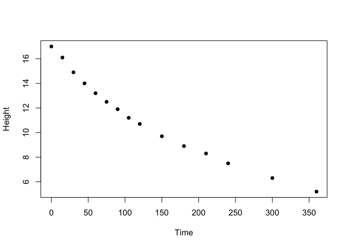
Figure 3.4: Scatterplot of foam height against time for the beer data.
The plot is strongly suggestive of a curvilinear (possibly quadratic?) relationship. We can fit the model with a quadratic term for time
\[ \color{red}{\text{Height}_i = \beta_0 + \beta_1 \text{Time}_i + \beta_2 \text{Time}_i^2 + \epsilon_i} \]
for \(i = 1, \ldots, 15\). This can be done in several ways in R. We will use the built-in function poly() to fit the model - note that this function automatically uses orthogonal polynomials which remove the correlations between the powers of the covariate completely, at the cost of interpretation but the gain of model selection. Fitting the model in R, we use the following commands:
We can summarise the model in the usual way (as it is still a multiple linear regression model):
##
## Call:
## lm(formula = Height ~ poly(Time, 2), data = beer1)
##
## Residuals:
##      Min       1Q   Median       3Q      Max
## -0.36021 -0.22760 -0.06058  0.25347  0.41401
##
## Coefficients:
##                 Estimate Std. Error t value Pr(>|t|)
## (Intercept)     11.16000    0.07612  146.62  < 2e-16 ***
## poly(Time, 2)1 -12.85980    0.29480  -43.62 1.37e-14 ***
## poly(Time, 2)2   2.96964    0.29480   10.07 3.31e-07 ***
## ---
## Signif. codes:  0 '***' 0.001 '**' 0.01 '*' 0.05 '.' 0.1 ' ' 1
##
## Residual standard error: 0.2948 on 12 degrees of freedom
## Multiple R-squared:  0.994,  Adjusted R-squared:  0.9931
## F-statistic:  1002 on 2 and 12 DF,  p-value: 4.442e-14
We see that both the linear and quadratic terms in time are highly significant beyond the \(0.1\%\) level. The \(R^2\) value is also very high, suggesting most of the variability in foam height is explained by the quadratic model in time. There seems little value in considering higher order terms in this case, but how do we choose in cases that are less clear-cut?
3.6.1 Choosing the order of a polynomial model
When dealing with polynomial regression models we now have an additional modelling question to consider - should we fit a quadratic, cubic, quartic or higher-order polynomial? As usual, we try to choose the simplest model which gives a reasonable fit. In practice, polynomials higher than a cubic are rarely used - practitioners would usually favour splines or a nonlinear model over a high order polynomial.
We start with a low order model and successively fit higher order terms until no significant improvement is obtained. Improvement is a subjective term, so this could be measured in terms of \(R^2\) (although other criteria may be better); in the special case of orthogonal polynomials this is made easier as each term in the model is independent. As soon as the highest order term becomes non-significant, then that term is unnecessary and model selection can finish. Once the order is selected, model adequacy should be checked in the usual way, i.e. residual plots, regression diagnostics.
Hierarchical model building
Consider the model \[ Y_i = \beta_0 + \beta_1 x_i + \beta_2 x_i^2 + \epsilon_i \]
for \(i = 1, \ldots, n\). Suppose we fit this model and find that the regression summary shows that the linear term is not significant but the quadratic term is. If we then removed the linear term, our reduced model would then become \[ \color{red}{Y_i = \beta_0 + \beta_2 x_i^2 + \epsilon_i.} \]
Suppose, however, we then made a scale change whereby \(x_i \rightarrow x_i + z\) for \(i = 1, \ldots, n\). The model above then becomes
\[\begin{align*} \color{red}{Y_i} &\color{red}{= \beta_0 + \beta_2 (x_i + z)^2 + \epsilon_i} \\ &\color{red}{= \beta_0 + \beta_2 z^2 + 2\beta_2 x_i z + \beta_2 x_i^2 + \epsilon_i} \end{align*}\]
The linear term has now reappeared and so our model has effectively changed. Scale changes (such as our mean-centering seen in chapter 1) should not make any important changes to the model, but in this case an additional term has been added, which is highly undesirable. We want our models to be scale invariant.
This illustrates why we should not remove lower order terms in the presence of higher order terms. Model building should be hierarchical and we do not want the interpretation of the model to depend on the choice of scale. Removal of the first order term here corresponds to the hypothesis that the predicted response is symmetric about \(x_i = 0\), which is not usually tenable and the same argument can be made about taking out the intercept term when it is not significant. Thus it also should be retained.